TL;DR: Word2Vec kickstarted the era of learned word representations by turning words into dense vectors based on their context, capturing meaning through proximity in vector space. This blog post breaks down its core ideas, architectures (Skip-gram & CBOW), and loss functions (cross-entropy vs. negative sampling).
The repsitory with the corresponding PyTorch implementation is available here.
Have you ever thought about how we teach machines which words are similar — and which ones aren’t? It’s wild to realize that our phones had smart autocomplete features decades before modern AI tools like ChatGPT became mainstream.
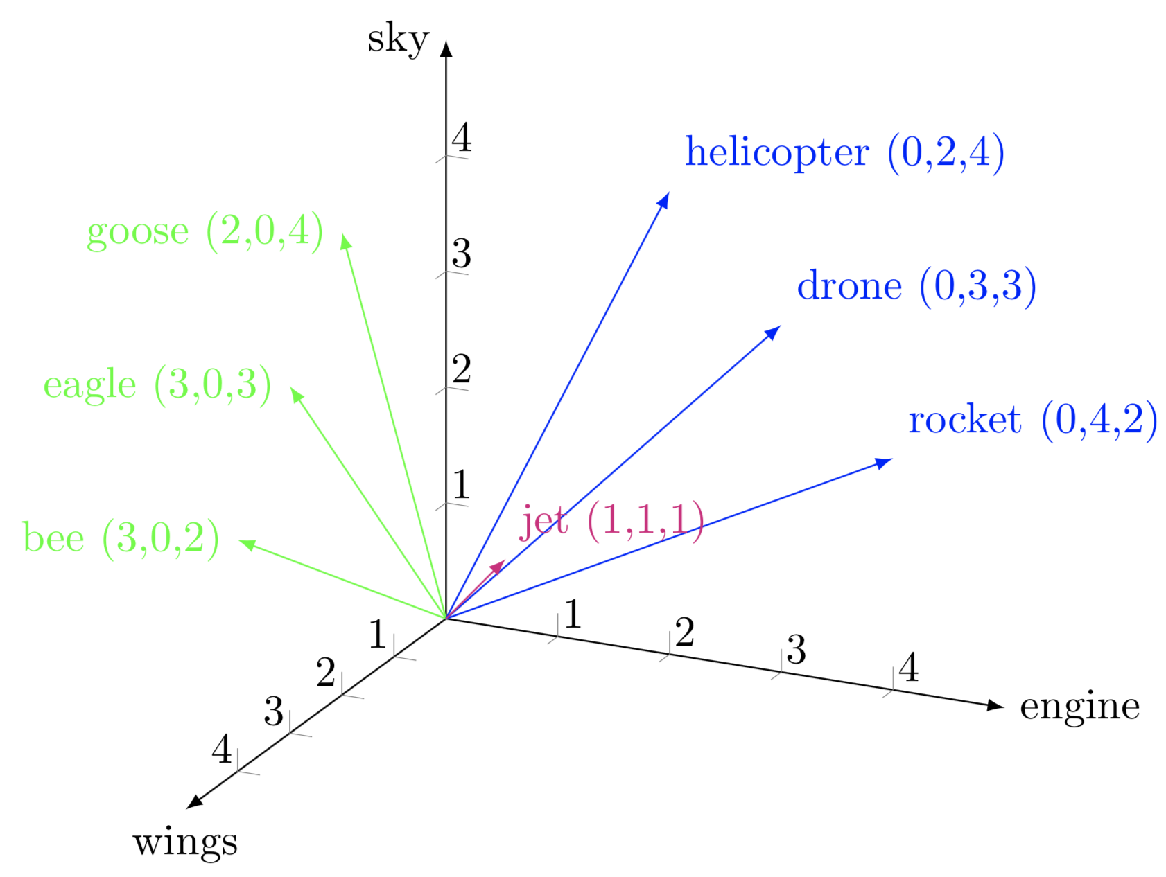
In a n-dimensional space, words “cling” to their own axes—Word2Vec learns this by pushing true neighbors together and pulling random words apart (this is a form contrastive learning, teaching the model to tell 'correct' context words apart from random ones).
Word embeddings laid the foundation for modern NLP models. Before transformer-style architectures took over (with their dynamic embeddings), Word2Vec was the go-to method for capturing the semantic meaning of words through dense (~ 100-300 dim) vectors.
In this post, I’m walking through the intuitions, architecture, methods, and math behind Word2Vec — and eventually implementing it from scratch using PyTorch.
What is Word2Vec?
As the name suggests, Word2Vec is a method to take a word and put it into a high dimension vector space. For example, we could see
dog = [0.03 -0.84 0.91 ... ] # 300 values
and that’s where the word “dog” would live in that space. The core idea behind creating Word2Vec is that words that appear in similar contexts should have similar representations and should appear closer together in higher dimensional vector spaces. This principle is often summed up as “you shall know a word by the company it keeps” and forms the foundation of modern embedding models. Instead of manually designing features, Word2Vec lets the model learn them by predicting words based on context.
There are two main ways to solve this problem:
- Skip-gram — Predict surrounding context words given the current word.
- Continuous Bag of Words (CBOW) — Predict the current word given its surrounding context.
In both cases, the model learns to assign each word a dense vector in a high-dimensional space — an embedding — such that semantically similar words are close together.
At the heart of the model is one hashmap and two embedding matrices:
-
Lookup Table - Maps words from your vocabulary to a number between
0andlen(vocab)-1➝ each one of those numbers represents a row in the embedding matrices -
E_in — Used to represent the input word
-
E_out — Used to compute predictions over context words
I used to get confused on why we needed two matrices because I always wondered why we couldn’t use just a single matrix.
The answer is that we need one embedding to represent the word itself and a second one to represent how it behaves as a context word. These turn out to learn slightly different properties.
Here’s an easy way to visualize a matrix like E_in or E_out.
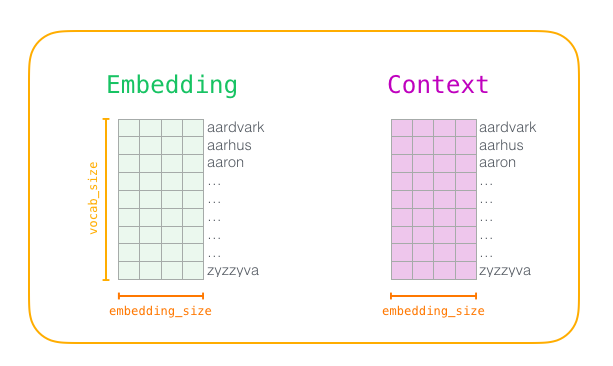
Both of these are matrices with the same dimensions but very different values (embeddings used to represent the input word vs. embeddings used to predict context).
Both are of shape (vocab_size, embedding_dim). During training, we take the dot product of the input word’s vector from E_in with all rows of E_out, yielding similarity scores. A softmax is typically applied to convert these into probabilities, and the model learns by maximizing the probability of true context words. After training, we often discard E_out and treat E_in as our final word embedding matrix.
Here, we are learning two embedding matrices, E_in and E_out which will contain dense vectors that have information about the semantics of our corpus. We also have a couple different ways to learn these matrices (skip gram, CBOW) which approach the problem in different ways.
Methods to approach word embeddings
The simplest way in training Word2Vec is first creating two matrices E_in and E_out and initializing them with Xavier. Formally, E_in, E_out ∈ ℝ^{|V| × d}, where |V| is the vocabulary size and d is the embedding dimension. Xavier initialization sets each weight to values drawn from a distribution whose variance keeps activations well-scaled, preventing gradients from exploding or vanishing—even in this mostly linear architecture.
For a quick recap / introduction to Xavier style initialization, I recommend reading this other small post.
Vanilla Training Method
The the most straightforward way to train Word2Vec is to use the full softmax across the whole vocabulary. Here’s how is works:
- Given a word, find it’s row index using your lookup table.
- Take the row index, grab its corresponding embedding vector from E_in (recall that each row in E_in is its own embedding).
- Compute dot products between this vector and every row in E_out, giving you a tensor of shape
(vocab_size,). - Apply a softmax over all vocabulary words to get probabilities of what are close. You have the option to sample top k here or just pick the argmax (in implementation I only used argmax).
- The model learns by maximizing probability of the true context word ➝ we must use cross-entropy loss.
- Backpropagate and update weights in both embedding matrices (E_in and E_out)
Pretty straightforward right? Here’s the catch:
Every forward pass, we are doing a softmax on your entire vocabulary, and your vocabulary might be around 50000+ words in real world datasets. Since only a small handful of words are related to any given word, most values (I’d say close to 98%) are going to be ~0 after the softmax. You are essentially doing thousands of unnecessary calculations per word pair, burning your compute and making training brutally slow, though the core weight updates are only from a small handful of words that you have.
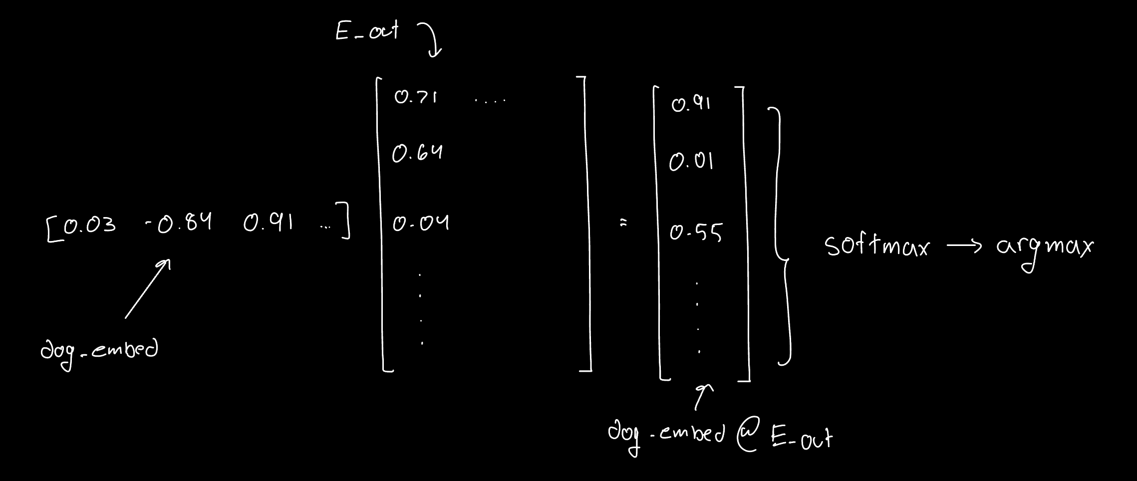
This is what's happening behind the scenes for a forward pass for the word "dog": dog_embed @ E_out ➝ softmax ➝ argmax
Bottom line: This method is great for understanding the core math/backprop and what exactly is going on in Word2Vec but falls short in reality (unless you have time and money to burn).
Skip Gram with Negative Sampling
This is the industry standard method for training Word2Vec.
We’re keeping the same goal (learn embeddings by predicting nearby words) but we are addressing the main bottleneck: the O(V) cost of computing softmax over the entire vocabulary on every forward pass.
What SGwNS says is
“Computing softmax over all 50000+ words in your vocabulary is too expensive. Let’s just compare the center word to 1 good (related) word (ground truth word) and take a random sample of bad (unrelated) words to push them away”
So we aim to maximize (and minimize) different things here:
- Maximize
σ(dot(E_in[center], E_out[context]))→ we want this close to 1 - Minimize
σ(-dot(E_in[center], E_out[negative]))→ we want these close to 0
Where σ is the sigmoid function, not softmax. We replace the softmax with sigmoid-based binary classification, scoring each (center, context) pair individually:
- One positive pair is scored and pushed closer
- k negative pairs are scored and pushed apart
This turns the multi-class classification problem into k+1 binary classifications, and the total loss is a sum of sigmoid-based log-likelihoods — way cheaper to compute and easier to train.
And this is exactly how we beat the bottleneck: contrastive learning.
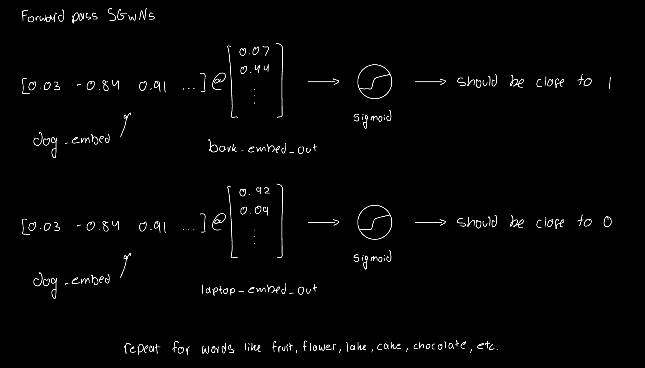
This is what's happening behind the scenes for a forward pass for the word "dog": dog_embed @ bark_embed_out ➝ sigmoid ➝ loss
Bottom line: We are using a smart trick to push away random words that are not meaningful to our current word, hopefully resulting in results similar to the vanilla method. (Spoiler: this trick does work really well and that’s why it is the industry standard)
Continuous Bag of Words
This essentially works in the opposite direction as Skip-Gram.
- Instead of predicting context from the center word, you predict the center word from it’s surrounding context words
- You take all the context word embeddings, average (or sum) them, and feed the result into the model.
- The model then tries to guess the center word using either of the methods we talked above:
- full softmax (like the vanilla version, we can expect a huge computation cost as before)
- negative sampling (like SGwNS)
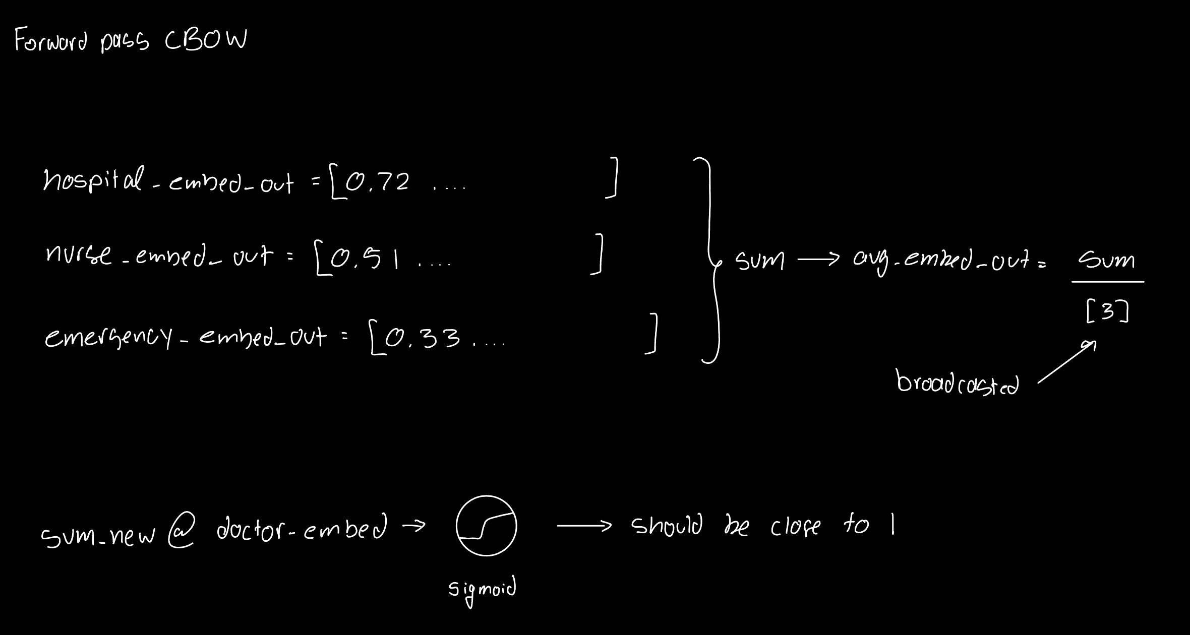
This is what's happening behind the scenes for a forward pass for the word "doctor": avg_embed_out @ doctor_embed ➝ sigmoid ➝ loss
Bottom line: Since we are comibing multiple context words into one average (or sum), CBOW trains faster than Skip-Gram and is more stable for smaller datasets. However, the main tradeoff is the fine-grained semantic realtionships because of that averaging. Most of the times, this method performs slightly worse than SGwNS and hence insn’t that big in practice.
Next, let’s talk about loss functions for each method.
Training Objective
Let’s split up the training objective by section and then we can ask two more sub-questions within each section:
- What should our loss function look like to actually pull together words that are similar (or push away words that are not similar)?
- What gradients flow back once we have a scalar loss?
Vanilla Training Method
Here, we want the model to assign high probability to the correct context word. We don’t care about other words right now - we just want:
- Low loss when the predicted context word is the actual neighbor
- High loss when the predicition is far off (e.g.,
coffeeshowing up nearbird)
Since this is a multi-class classification task (predict 1 word out of vocab_size), the natural choice is to use cross-entropy loss applied on top of a softmax.
The Goal:
Maximize the probability of the true context word $w_o$, given the center word $ w_c $: $$ P(w_o \mid w_c) = \frac{e^{u_o^\top v_c}}{\sum_{w=1}^{V} e^{u_w^\top v_c}} $$
Math symbols scare me too so I’ll break down what that it saying. The numerator measures how close the correct word is to the center word (via dot product). The denominator compares the center word to every word in the vocabulary. So if $w_o$ is genuinely close to $w_c$, we get a large numerator. If a bunhc of irrelevant words are also close, we would have a large denominator.
We want to maximize this probability so that means making the true word similarity as big as possible while keeping all other dot products in the denominator small. In this case, cross-entropy loss is the star.
It’s defined as:
$$ L = -\log\ \Bigl( \frac{\exp(u_o^T v_c)} {\sum_{w=1}^{V} \exp(u_w^T v_c)} \Bigr) $$
This basically measures “how surprised are we by the correct answer?”, exactly what we should be asking when we predict a good/bad word. We now have a scalar loss that we can backpropagate through our network (with loss.backward()).
During backpropagation, only the embeddings of the center word and the true context word actually get updated. All other words are just there to normalize the softmax, they aren’t contributing anything else. This is why is method is so inefficient - we are doing a HUGE amount of computation just to update 2 weights (crunching 50k numbers to update 2 weights).
Let’s fix this O(V) nightmare in the next section with negative sampling.
Skip Gram with Negative Sampling
First, here’s some terms that we are going to be referencing
- $\sigma(x) = \frac{1}{1 + e^{-x}}$ is the sigmoid function
- $u_o$ is the embedding of the true context word (positive)
- $u_i$ are the embeddings of $k$ negative words
Let’s address this bottleneck now. Instead of predicting one word out of 50k, we can turn it into a binary classification task.
True context word → label it 1
Random (irrelevant) word → label it 0
For every center word, we train on:
- One positive pair (center, actual context word)
knegative pairs (center, randomly sampled “noise” words)
And we are going to use the sigmoid function here instead of softmax so that each pair is treated independently.
Probability Objective:
We want to maximize the probability that a real word pair appears together:
$$ P(\text{real} \mid w_c, w_o) = \sigma(u_o^\top v_c) $$
And for a negative (fake) sample, we want to minimize:
$$ P(\text{fake} \mid w_c, w_i) = \sigma(-u_i^\top v_c) $$
Unlike softmax, which compares all words at once, sigmoid allows us to independently judge each word pair, making negative sampling scalable.
Loss Function:
$$ L = -\log(\sigma(u_o^\top v_c)) - \sum_{i=1}^{k} \log(\sigma(-u_i^\top v_c)) $$
This is a really cool loss function because it has two jobs. One for pulling the true word closer together and one for pushing the fake words away. We can see that the first term is calculating the negative log of the similarity between the center word and the context word. This gives us a loss that is lower when they are highly similar - exactly what we wanted.
The second term is where we pull in embeddings for k negative sampled words that are not in the context. We want their similarity with the center word to be low - that’s why we negate the dot product, apply sigmoid (which favors small similarity), and penalize high values. In a nutshell this pushes away random/fake context words, minimizing the chance that the model falsely thinks they belong together.
These two terms combined teach the model “pull what matters, push what doesn’t” without ever needing to score the entire vocabulary. Just enough positive and negative contrast, and the model figures out the structure of language from there.
A small side note: this loss function does multiple things at once which is very iconic in machine learning. This type of loss function made way for things like GAN loss, VAEs, and Multi-objective losses.
Continous Bag of Words (CBOW)
You probably get the gist of what we do now: understand our probability objective and based on that, make a loss function.
Here, we have to be ready to flip our heads in the opposite way. We are going to predict the center word now, given a set of context words.
The probability objective:
$$ P(w_c \mid w_{c - m}, \dots, w_{c + m}) = \frac{e^{u_c^\top \bar{v}}}{\sum_{w=1}^{V} e^{u_w^\top \bar{v}}} $$
Our loss function (with negative sampling) is:
$$ L = -\log(\sigma(u_c^\top \bar{v})) - \sum_{i=1}^{k} \log(\sigma(-u_i^\top \bar{v})) $$
- $\sigma(x) = \frac{1}{1 + e^{-x}}$ — the sigmoid function, which squashes scores into a range between 0 and 1. We use it to convert similarity scores into probabilities.
- $u_c$ — the output embedding of the center word (the word we’re trying to predict). Think of this like a “target” vector.
- $\bar{v}$ — the average of the input (context) embeddings surrounding the center word. This is what we feed in to predict the center.
- $u_i$ — the output embeddings of $k$ negative samples (randomly chosen words that are not the true center). We want the model to push these words away from the context representation.
Main tradeoffs
We’ve seen that Word2Vec is powerful for learning dense, meaningful word embeddings from raw text — but it doesn’t come without limitations. Here are the key tradeoffs baked into its design.
Corpus sensitivity
In Word2Vec, everything is solely based off the co-occurrence statistics of words.
- A model trained on Shakespeare will associate words like thy and alas, while a model trained on Reddit/Twitter would lean towards bro and lol.
- The model reflects and amplifies the biases, slang, and domain of the data it sees
Static Embeddings
As we could see, each word gets only one vector.
- The word bank will have the same vector whether you are talking about a financial institution, a riverbank, or even in slang how people say a lot of money is “bank”
There’s no ability to disambiguate meaning based on context.
No OOV Handling
Out of Vocab (OOV) is huge in language processing because in the real world, language is messy and spoken in many different ways. Word2Vec creates embeddings only for words seen during training.
- If a word doesn’t appear in the corpus (look up table returns a null value), there’s no embedding and hence no meaning (even if it’s just a slight verb change: happy ➝ happier)
This is very brittle in the world where vocab drift happens on a daily basis.
Local Co-occurrence ≠ True Semantics
Word2Vec assumes words that appear together share meaning but this just isn’t true in some cases.
- Doctor and death might be close to each other if our window size is not that small, but our model would now relate these two words whereas they are complete antonyms.
In general, Word2Vec struggles with antonyms a lot.
Hyperparameter Sensitivity
Results can vary significantly based on their
- Window size
- Negative sampling rate
- Embedding dimensionality
Especially when training locally (where a single epoch takes foever), tuning these can be very tedious and time consuming.
Coding it out
My repository is structure as the following
word2vec-project/
├── data/
├── models/
├── notebooks/
├── train/
│   └── train.py
├── visualization/
│   └── visualize_embeddings.py
├── word2vec/
│   └── word2vec.py
├── dataset.py
├── debug_dataloader.py
├── load_data.py
├── utils.py
├── visualize_embeddings.py
├── README.md
├── requirements.txt
└── .gitignore
the README contians the eval differences between the vanilla method, SGwNS, and CBOW where the differences in accuracy and training time are reflected clearly.
Conclusion
Word2Vec may be old school now, but it’s still one of the most elegant and interpretable ideas in the NLP world. I really like it because it’s a great way to build up your ML intuition, understand the baby steps towards contrastive learning, and the results reflect the theory very well.
If you enjoyed reading this feel free to star this repository on GitHub!